
Kepler Orbit Demo
In one of my previous posts (Available HERE), I was using numerical math to create a real-time 2D simulation of moving objects by taking into account Newton’s laws of motion and the Newton’s law of gravity. The simulation was powered by several methods for solving Ordinary systems of differential equations, including the most basic Euler Method and followed by some advanced methods, such as Runge-Kutta 4th order. This numerical model has however several disadvantages over a real motion of those objects.The first thing to note is that it is not accurate. Its accuracy largely depends on the used data type for computation, discretization in time and the method used for estimating the planetary movement (as well as some other factors). This time,I have decided to use Kepler’s laws of planetary motion to model those movements.
In fact, we will take a short look at the basic concepts already known. An object with relatively small mass in comparison with the central body (For example Sun and Earth) is orbiting the body on some kind of a conic curve. This can be either a circle in the ideal state, but most likely on an ellipse – with an elliptical orbit. In case the object comes from the outer space and has a huge velocity, it can draw a paraboloid or hyperboloid. This usually means that the object is just passing through the central body’s gravity field and its direction is slightly changed during this time. Anyway this situation is not of our interest, so we will further concentrate on the elliptic movement

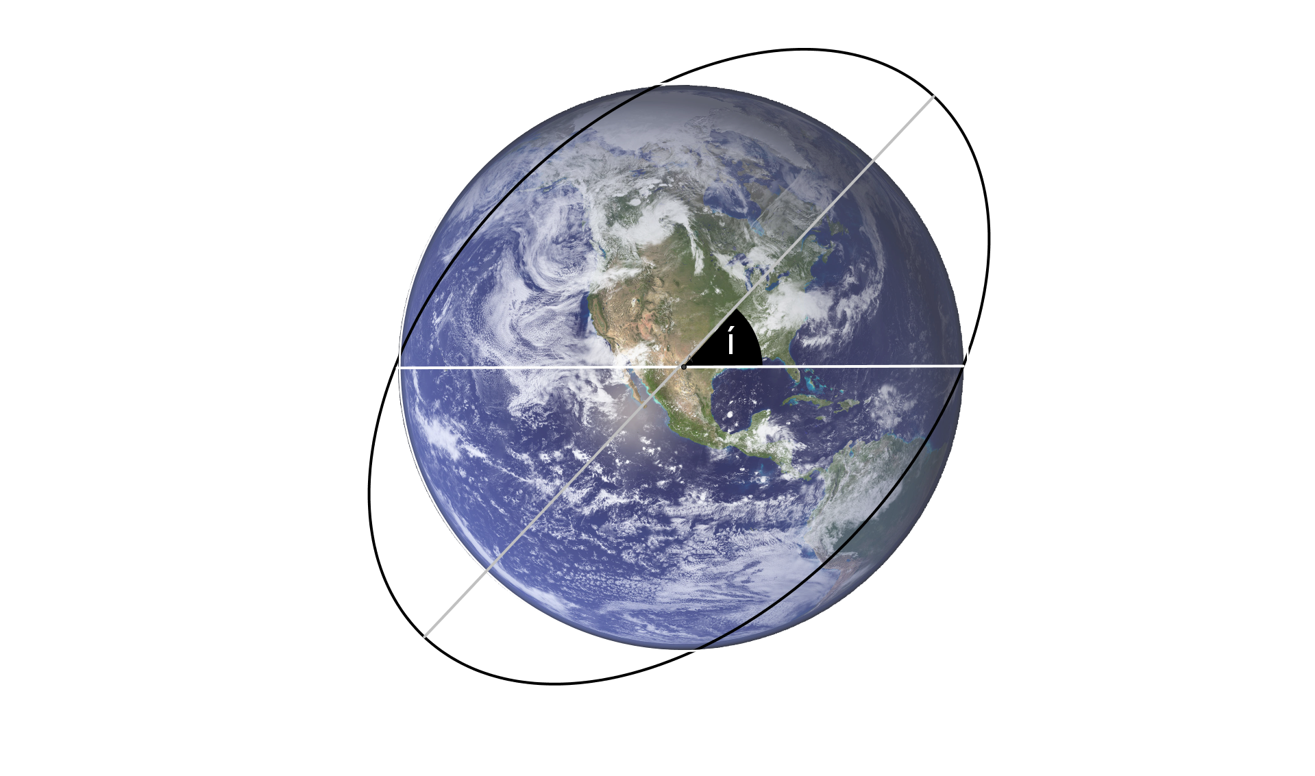
To describe an ellipse, one has to know its Major Axis (a) and Minor Axis (b). If these 2 are known,the eccentricity of the ellipse can be computed. Please note that in case of circle, a is equal to b,thus eccentricity is zero. The first of the Kepler’s laws states, that the planets are orbiting the sun, which lies in the focus of the ellipse, which is self-explanatory. Now the second Kepler’s law states, that the closer the object is to the central body, the faster it travels. Eg the area swept by the object as it moves closer to the body is equal to the area when the object is located farthest from the body. The reason is that when its moving close to the body, it moves fast and the distance to the central body is low. On the other hand, when the object is far away, it moves slowly, but the distance is huge. This is depicted on the following image.

The area units are not important right now. The third Kepler’s law relates the orbital period to the major axis such that the square of the period is proportional to the cube of the major axis. This ratio should be constant for all planets. The formula is depicted on the image below. Now because so far, I have talked about planetary motions, I would like to mention that there is no difference in the movement of the planets around the sun and in the movements of the satellites on the sky. This is due to the fact that in both cases, the orbiting objects’s masses are a fraction of the central body’s mass.

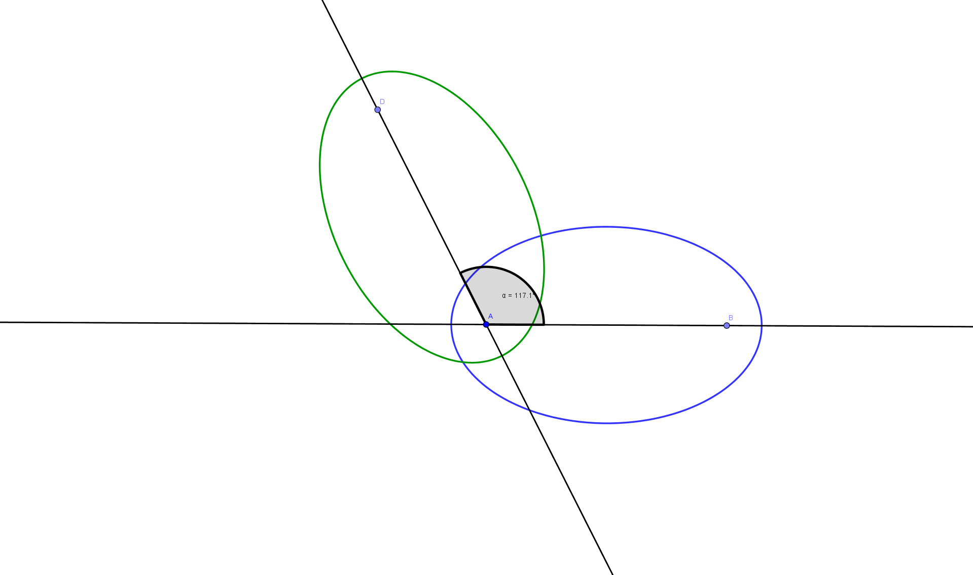
As we know, these movements are periodic, which means, that they do repeat just like summer repeats each year. If we can somehow figure out the relationships, we could be theoretically able to predict or compute the position of any orbiting object in arbitrary time. In fact this is where the Kepler’s laws take place. There are 6 Keplerian parameters , which exactly specify the position of the object. As it was mentioned before, 2 are connected to the ellipse itself: the Major (a) and Minor (b) axis of the ellipse (Or Eccentricity, because it is related to a & b). 3 Additional parameters specify the position of the ellipse in 3D space to a reference plane (The Earth’s equatorial plane for example). At first, it is the so called Ascension, which rotates the ellipse around the Z axis. Thus Ascension can range between 0 and 360 degrees. The second one is the Inclination ,which rotates the ellipse around the Y axis. Range for this parameter is -90 to 90 degrees. The last one is the Perilapsis, which is in turn the rotation of the ellipse around the the last X axis. The range is similar to the Y axis. The last 6th parameter is called the true anomaly,but its nothing more than a position of the object at a specific time. The next 2 Images should explain the Ascension and Inclination of the ellipse.
One of the most famous equations (Kepler’s equation) however is the formula for estimating the Eccentric anomaly (E). M = E – e.sin(E). This equation cannot be solved analytically. This is where numerical methods are of great use once more. In fact solving this method numerically is easy to implement and whats more, it converges usually fast (While using Newton’s method) . To sum it all up, we have to know 6 Keplerian parameters : a,e,Ω,ω,ι and t. Then we can compute the Mean (M), Eccentric (E) and True (v) Anomaly along with the distance vector r. The last thing to do is to (optionally) transform results into Cartesian / Polar coordinate system. Please note that I prefer to talk about angles in degrees, however goniometric functions are usually implemented in radians.
XData = r*( cos(Ascending)*cos(Perilapsis + v) – sin(Ascending)*sin(Perilapsis + v)*cos(Inclination) );
YData = r*( sin(Ascending)*cos(Perilapsis + v) + cos(Ascending)*sin(Perilapsis + v)*cos(Inclination) );
ZData = r*( sin(Inclination)*sin(Perilapsis + v));

By default, the simulation includes 3 satellites with randomized 6 keplerian parameters, Each of their trajectory can be visualized by drawing a custom surface (Possibly also with an equatorial plane) in the 3D. Since the only requirement of how to calculate the satellite’s position is time (IE. no need to know last position and speed of the satellite), the time scale can be easily adjusted – discretization in time is therefore irrelevant. Furthermore, no error actually accumulates over time. The computational error is within the precision of those parameters.
As always, the demo is available ➡️ HERE ⬅️ 🐾