
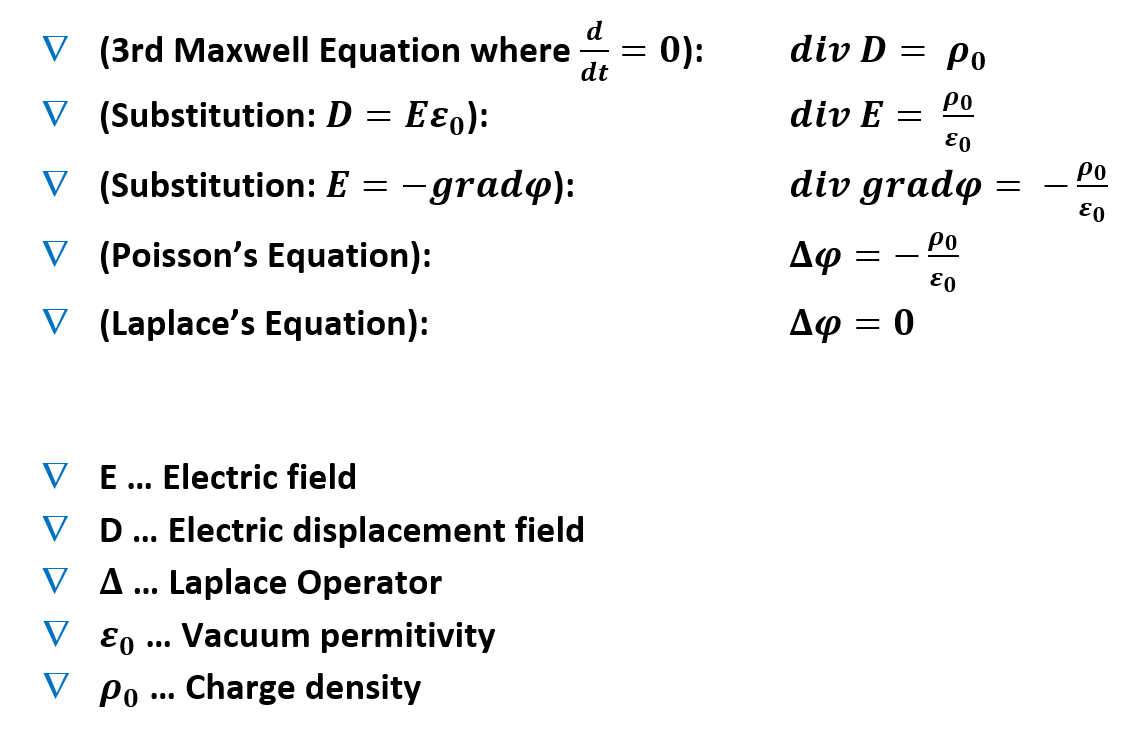
Back at the university, I got excited about one of the methods used for computing various quantities from electro magnetics. Particularly the method of finite differences, which is not among the widely used methods, but is somewhat simple to understand and compute (Its not the most efficient method either – but it can be easily accelerated by CUDA). It can be used to calculate the distribution of electric field within a well-defined shape such as in a waveguide.The method uses the Laplace’s Equation deduced from the third Maxwell’s Equation when d/dt = 0 (Static Field) and is a special case of the Poisson’s equation without any free charges in space. Used derivation is depicted below:
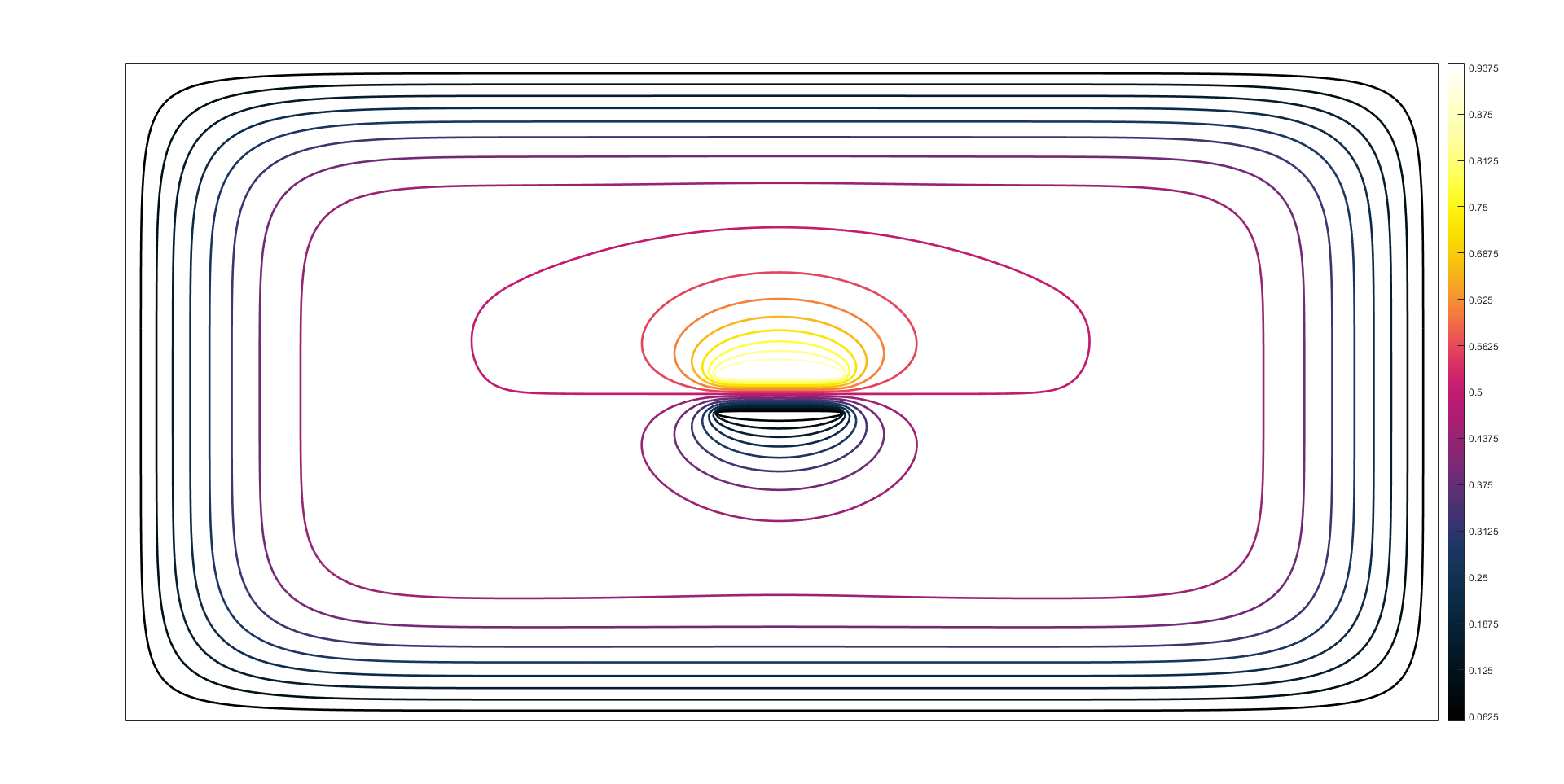
The Idea behind this method is quite simple. The area of interest is discretized into a (Usually) rectangular grid of points with a distance between them of “h”. Inside the grid, we define the initial conditions such as voltages on various surfaces (IE Borders of the waveguide or voltages of microstrip lines) These are known to be “Dirichlet Conditions“. However we would like to calculate the distribution of the field (The Electric Potential φ) in the discretized area. There is a method to directly solve the problem via matrix inversion, but due to additional complexity, it is usually solved iteratively with one of the popular methods (Jacobi, Gauss-Seidel, SOR).
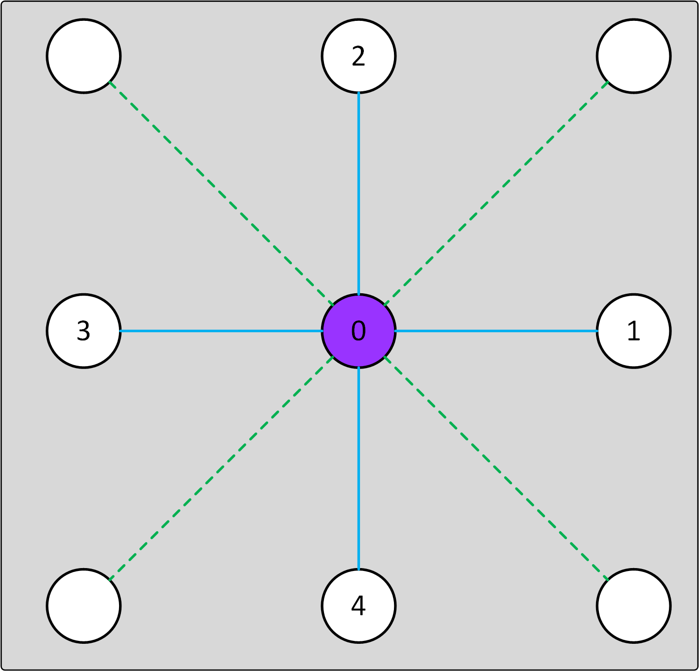
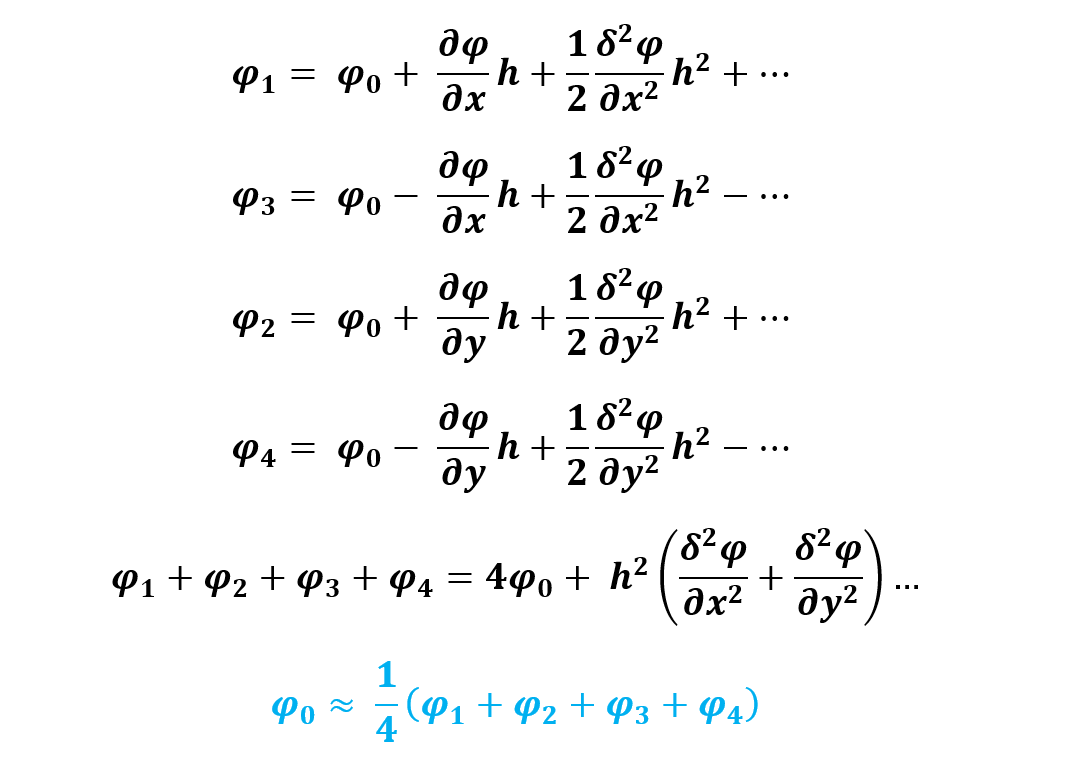
From the Laplace’s equation, we are just close to the formula used in the FD method. We approximate the differential operator in 2D space (although this can easily be extended to 3D problems as well) via the Taylor expansion. Please note that I have added green diagonal points, which are at distance sqrt(2) but are not required for the deduction of the formula. Their purpose is to test their influence on the convergence of the methods used later.
The whole problem just therefore shrinks to updating nodes until the difference between iterations Is small enough so that we can say its accurate to our needs. The only problem comes after realizing that these grids are usually large and the convergence of such grids is slow simply due to fact that if there are 2000 points in the X direction, it takes 2000 iterations for the points in the corners to actually make some evidence about potential on the other side of the grid. There are 3 commonly used iterative methods used for solving of this problem: The Jacobi Iteration, The Gauss-Seidel Method and the Successive Over Relaxation (SOR) Method. The Jacobi method is the easiest method with the longest convergence. It calculates the residuum for each point of the grid and updates the grid after all points have been calculated. Therefore it also requires 2 times as much memory, which may be a problem in some cases. On the other hand, the Gauss-Seidel method doesn’t require additional memory, as it updates the grid points on the fly (Eg. point at x = 3 uses values from point x = 2 directly after point at x=2 has been computed.). According to Computation Electromagnetics , it is however necessary that the grid is updated this way with increasing I and j (x and y dimension). This is not a problem for a CPU-based implementation, but will instantly kill any CUDA – based approach.
The latest method is a modified method of the Gauss-Seidel method with a parameter called “Super Relaxation Coefficient ω” which tends to vary in range from 1.0 to 2.0. Value of 1.0 is equal to the Gauss-Seidel method and value of 2.0 or more leads to divergence of the method (Don’t use or just give it a try!). The goal of this parameter is to guess the value in the grid faster by applying “more” of the calculated residuum or correction to the next iteration per point. I have reprogrammed the algorithm to CUDA and included the SOR coefficient to the “Jacobi Iteration”. The results are such that when SOR is < 1,the algorithm is convergent (The closer to zero, the longer the convergence), however when above 1, it starts to diverge. Here is the only plus for the 8-grid option, as when the coefficient is approx 1.3, then the 4-grid option diverge while the 8-grid method is convergent anyway and requires less iterations to finish (Although each iteration is more costly). When the coefficient reaches sqrt(2), even the 8-grid algorithm diverge. Overall the benefit of using the 8-grid is negligible.
The method can be made more generic by adding proper calculations in areas with different permittivity in the area of interest – This is so far not implemented and the microstrip lines in the example “levitate in the air“. Normally there would be a substrate around with different permittivity. In order to further speedup the calculation, the convergence criterion can be skipped at a cost of computing fixed amount of iterations. Because this task is natively suited for GPU architecture and relatively easy to understand, it exhibits approximately 20x speedup over Matlab CPU implementation (Will vary based on CPU and GPU). In theory, the computation can be even faster by taking advantage of the shared memory (Also not Implemented).
Project CODE can be downloaded ☄️ HERE ☄️ and contains Matlab scripts for visualizations as well as VS 2019 project for compilation of a mex file.