I have decided to create a small introduction to the concept of using fixed point representation in FPGA for DSP Operations. Because naturally in RTL design (VHDL, Verilog), there is no standard data format such as “integer or float”, but only logic vector with bits representing the data (Ommiting now also the numeric libraries found in verilog and VHDL), its always a good idea to negotiate and or describe the data formats at the input of some DSP processing block and as well on the output of such a block. The most important part is to actually understand the concept of 2’s complement data format, which may represent both signed and unsigned values. From my experience, it is usually a good idea to not mix signed & unsigned formats at once and use only one of them. Under most circumstances, this will turn into signed 2’s completemnt usage (With exception on some video processing tasks for example).
The very first thing, that needs to be clear at the beginning is the notation for the format. I do use the notation Q.X.Y. In this notation, X is a number of bits for the dataword. This would be for example 32 for integer values. Y then specifies how many bits of the LSBs are used for fractional part of the number or where the binary point lies to be more accurate. For example signed Q8.5s number means the following: the first bit is the sign bit “s“, the second and third bits are the “integer” bits, which may indicate that the signal’s magnitude may be in range from -3 to 3 [bit2 == 21, bit3 == 20] and the rest are the fractional bits of the number, which as well contribute to the magnitude : [bit4 == 2-1,bit5 == 2-2, bit6 == 2-3,bit7 == 2-4 and bit8 == 2-5]. In case all the fractional bits are ones, this would indicate the value of: [0.5 + 0.25 + 0.125 + 0.0625 + 0.03125 = 0.96875]. Therefore in this format, the maximum value is the sum of the integer and fractional parts: 3 + 0.96875 = 3.96875.
Although there are occasions when more integer bits are needed, such as high gain scaling (Gain > 0dB), or computation of and absolute value of a complex number (this may have a magnitude of sqrt(1+1) = 1.4), I mostly tend to use the format of QX.X-1, in which there is no integer part of the number, but instead all bits represents the fraction. Therefore the fractional range lies from -1.0 to 1.0. In this format, the computation of the absolute value of a complex number cannot be done, since it may eventually overflow, as the theoretical maximum may be up to 1.4, which is more than the format QX.X-1 may represent.
There is also a slight difference between reinterpretation of the signed/unsigned data in this format. In unsigned format, there is no sign bit and thus Q8.7u unsigned would have 7 fractional bits, but also 1 integer bit. In comparison, signed Q8.7s would still have 7 fractional bits, but since the first bit is the sign bit, then there would be no integer part. The maximum ranges for these formats therefore differ (2.0 for unsigned,1.0 for signed). Note that neither of those values may actually reach 1.0 or 2.0 exactly due to limited precision.
Floating Point Conversion
As with every data format, there is a need to specify the conversion rules to other data types. Among them, the mostly used is the conversion to/from the floating point values (either in single or double precision). Conversion from floating point to fixed point is simple as its inverse. Val_Fixed_Int32 = Val_FP * 2Num_Frac_Bits . Because integers are naturally 2’s complement as well, the integer value may be written to a databus in the int32 format. For example conversion of π to Q16.13s would be: Pi_Fixed_int32 = 3.14*213 . This is 25736 in 32-bit integer or “0110010010001000” in binary. The green zero specifies that the number is positive, red ones indicate magnitude of 1+2 = 3 and the blue fractional parts are the fraction, which should be 0.14, so together 3.14. The conversion to floating point is similar. We read the value as an integer and scale it down to match the fraction length: Val_FP = Val_Fixed_Int32 / 2Num_Frac_Bits. For example “0101011011111100” in the same format reads as 22268 in plain int32. We divide it by 213(8192), so that the result is 2.71826171875, which is surprisingly the euler number exp(1).
Truncation / Rounding
The simplest operation, which costs nothing in the hardware at all is truncation. Truncation means, that we are discarding some bits of the signal we don’t want. These can be usually either LSBs or MSBs. There is however one problem caused by truncation, which is the creation of the DC bias in the truncated signal. This may be easily verified for example in Matlab. Because the DC is “very small” I do the checking at the zero frequency in spectrum via FFT, although it may also be done by computing the mean of the signal. DC Bias may be a problem, because it might just lead to wrong detection of other signals and or reduce the dynamic range of a signal in case high gain scaling is needed.
In order to overcome DC creation, the bits, which should be in the previous scenario truncated, are instead used during rounding to decide whether the dataword should be increased or decreased in magnitude by the dataword’s LSB. Rounding therefore consists of comparison of the “truncated” bits to a constant and then of an add/sub operation. In case of using 32-bit datawords, this means a 32-bit adder. That is why rounding is not extra efficient operation in hardware. In case of rounding 16+LSB bits,the comparison may also become a timing problem in FPGAs for higher clock frequencies. Fortunately both operations can be pipelined. Below is an example of a test signal consisting of 2 sine waves and noise in format Q16.15s,which is truncated “violet” and rounded “green” to Q8.7s. The DC is approx -33dB for truncation and -87dB for rounding,which is a 54dB difference.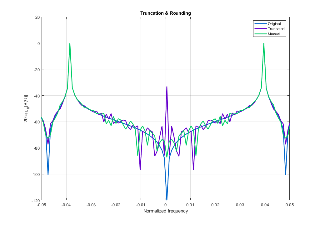
Bit Extension
There are basically 2 types of extensions based on what we want and from which end of the dataword we add the missing bits. The extension can therefore mean: LSB extension (adding bits to the right of the LSB) or MSB extension (Adding bits to the left of the MSB). Working in unsigned format is simple, since in both cases, we add zeros to the signal. However what is not as easy to see is that when we use the unsigned format for the fractional data, it depends on which end of the word the zeros are added. For example,taking π/4 in Q8.7 unsigned ( ‘01100101‘ ) and extending the word with LSB zero extension to “01100101 0000” leads to format Q12.11. In this notation, we just added to the original number a value of: 0*2-8 + 0*2-9 + 0*2-10 + 0*2-11. This is of course still the same value (π/4), which is the result we usually want when we do an extension. The second option is to use MSB extension to “0000 01100101“. In this case,we have just created a number with format of Q12.7 unsigned ,eg. we have left the fractional bits by the LSBs and added integer bits with the following values: 0*21 + 0*22 + 0*23 + 0*24. In this representation, the original value is still intact, which again is the wanted behavior. Now things gets a little bit more complicated when we use signed values as in this case, we need to sign extend the MSBs. Now please note that in case of signed values, MSB extension is done via Sign extension (In case the value is positive, the MSBs are extended with zeros while in case of a negative value, the MSBs are extended with the sign bit – ones). The LSBs however needs to be extended with zeros as well in case of a signed number. Therefore LSB extension (increasing amount of fractional bits) is always done via zero-extension.
Saturation / Overflow
Overflow doesn’t just happen randomly, but only if we try to reduce dataword width somehow. I do prefer to work mostly in full precision and do the required rounding/truncation/saturation after all the required operations have been done (given a reasonable bit growth for the digital part). For example, using a full precision on the output of multiply operation can never lead to overflow. The same applies for all mathematical operations on the data streams. if we have A = Q16.15 & B = Q16.15, then the correct output format, which cannot overflow during add/sub is Q 17.15. Eg each add/sub operation increases the required bitwidth of 1 bit. During multiplication, the full precision bitwidth is the summation of the bitwidths of the 2 operands.The same also applies for the resulting fractional length during multiplication. For example Q16.15 * Q8.7 = Q(16+8).(15+7) = Q24.22.
As I mentioned however, there is always a need to reduce the datawidth from time to time. In this case, we may discard the MSBs and or LSBs. The discarded MSBs may then cause an overflow while discarding LSBs leads to DC bias creation. For example, a value of 0.7 in Q8.7s has a binary representation of “01011010”. If we remove the MSB, the number becomes “1011010”,which is a negative number – it has overflown. We can also say, that the discarded MSB is in fact the left shift by 1 or multiplication by 2 in other words. So that if the number was 0.7 and the maximum representable number for QX.X-1 is 1.0, we definitely knew that it will overflow as 0.7*2 yields 1.4,which cannot be represented in QX.X-1.
Therefore overflow happens if we change the sign bit during truncation of the MSBs. The first bit after truncation must remain the same as before truncation, so that we known that overflow has not happened during truncation of the MSBs. If the MSB bits differ, we know that there was an overflow. In this case, we may substitute the truncated result for a number, which is either the maximum “011111…” or minimum “1000…” in the truncated format. This is saturation. As can be seen,saturation is easy to implement and basically consists of a few muxes and vector comparison with the truncated bits. The method was implemented in Matlab for checking functionality. Result is shown below.

Add/Sub Gain and data interpretation
As I have stated previously, given 2 numbers A(Q8.7) and B(Q8.7),the result after addition would have format Q9.7. For example: A(0.25),B(0.125),C = 0.375. In Binary A(“00100000”) + B(00010000) = C(“000110000”). Because we have used the same data formats for both operands,we may write A + A = 2A and say, that the gain of such an operation is equal to 2.0. As a result, we may just shift the binary point by 1 bit left. This is in fact equal to division by 2. This modifies the output format to Q9.8. In this format, value C becomes 0.375/2 = 0.1875.What is really interesting about this operation is, that in real hardware, nothing happens except 1 bit is added to the data vector. We can do so however only because we know that the gain of this addition is 2.0 and thus we can scale by 1 bit and compensate for the growth. This operation would be invalid, if we would use 2 different data formats. For example Q8.4 + Q8.6 = Q11.6 (Amount of fractional bits is equal to the maximum among the fractional bits of those operands and the integer part is taken from the number, which has more integer bits – This is Q8.4 (3 Integer Bits), which is then increased by 1 and one sign bit is added = 1(sign bit) + 3(orig int bits) + 1(new int bit) + 6(fractional) = 11 total bits). The maximum magnitude of operand A is 2.0,while its 8.0 for the second one. The first has therefore gain of 1/4 in comparison to the second operand (1.0) and the total gain of the addition is only 1.25 (2A + 8A = 10A – normalized to the gain of the second operand: 10/8 = 1.25). Using different data formats for the adder therefore need to be treated with special care.
Multiplication Gain and data interpretation
As I mentioned earlier during saturation, the result after multiplication should have the format specified as the sum of the integer and fractional lengths: Q16.15 * Q8.7 = Q24.22. What may be strange in the first place is that both operands use the QX.X-1 format,in which the maximum representable value is 1.0. The question is,why would we need another integer bit if we know that 1.0*1.0 is still 1.0? In other words, it seems like we could use the same format at the output. Well the simple answer is that we unfortunately can’t. Now lets see why: the maximum positive representable value for QX.X-1 APPROACHES 1.0,but in fact is 0.5+0.25+0.125+ …. and thus the positive value can never really be 1.0. In fact, if both operands are positive, the mentioned format could be used. It could also be used in case any one of the operands is negative. But it cannot be used if both operands are negative. This is because in 2’s complement, the ranges for positive and negative values are non-symmetric. As a result,-1.0 is representable in this format while 1.0 is not. Now if both operands would would have a magnitude of -1,then the result would be equal to: [-1.0 x -1.0=1.0]. As was just mentioned,1.0 cannot be represented in QX.X-1 and thus there is the need for the extra bit.
Most of the time however, carrying 1 extra bit along a 16 | 24 | 32-bit bus just because one of all the possible combinations on the data bus [(1/(216) | 1/(224) | 1/(232))] may be a value of -1 seems like a waste of resources. Unfortunately for fail-safe applications, we cannot just discard the bit,as it will or may cause an overflow. I would however say, that using saturation and safely discarding this bit is highly recommended for a good design and efficiency of the used FPGA resources.
A good – practise based on my experience is to always shift, saturate and round the result after each multiplication to the QX.X-1 as using several different data format across the design causes inconsistency and more likely leads to misinterpretation of the data and possible errors. However note, that QX.X-1 may be used only in scenarios, where the total digital gain is lower than 1.0. For example: We have a first stage decimation filter, which has a digital gain of -3.5dB. We may use a scaler with a gain of 3.5dB to compensate for this loss without any problems and use the QX.X-1 data format. Increasing the gain further would however lead to overflow (or saturation).
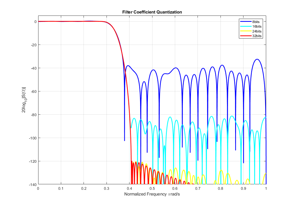
FIR Filter Coefficient quantization
There is quite a common question regarding FIR filtering – how many bits do I need for my FIR filter to have attenuation at least X dB in the stopband? You may be surprised, but the answer is not as simple as it may look. Especially because amount of bits is not the only thing, that is important. Having a lot of bits per filter coefficient is useless if the data format they use is chosen badly. For example, most applications use Low-Pass filters. A very specific feature of these filters is that the maximum coefficient value for these types is equal to the cut-off frequency of the filter. This means, that a filter, with normalized Wn = 0.5 would have the magnitude of the biggest coefficient equal to 0.5. If we chose the frequency as 0.125, then the coefficients’ maximum value would be only 0.125. This is important,as in the QX.X-1 format, this means that the first bits will become zeros and will be useless for the filtration.If the data format is chosen wisely,then the calculation is quite simple,as there is 20*log10(2) = 6dB attenuation in the filter stop band per bit. The example below uses the kaiser window to increase the stopband attenuation, which was defined as -120dB. The Normalized cut-off frequency (Wn) for the following example was chosen to be 0.33. Coefficients are in signed QX.X-1 format, although more accurate design would use QX.X to utilize even MSBs of the filter coefficients.